Simple Ornstein-Uhlenbeck Models

Estimating Evolutionary Optima

This tutorial demonstrates how to specify an Ornstein-Uhlenbeck model where the optimal phenotype is assumed to be constant among branches of a time-calibrated phylogeny (Hansen 1997; Butler and King 2004). We provide the probabilistic graphical model representation of each component for this tutorial. After specifying the model, you will estimate the parameters of Ornstein-Uhlenbeck evolution using Markov chain Monte Carlo (MCMC).

Ornstein-Uhlenbeck Model

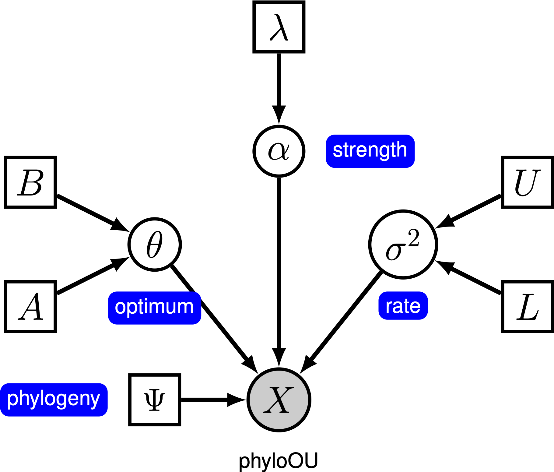
Under the simple Ornstein-Uhlenbeck (OU) model, a continuous character is assumed to evolve toward an optimal value, $\theta$. The character evolves stochastically according to a drift parameter, $\sigma^2$. The character is pulled toward the optimum by the rate of adaptation, $\alpha$; larger values of alpha indicate that the character is pulled more strongly toward $\theta$. As the character moves away from $\theta$, the parameter $\alpha$ determines how strongly the character is pulled back. For this reason, $\alpha$ is sometimes referred to as a ‘‘rubber band’’ parameter. When the rate of adaptation parameter $\alpha = 0$, the OU model collapses to the BM model. The resulting graphical model is quite simple, as the probability of the continuous characters depends only on the phylogeny (which we assume to be known in this tutorial) and the three OU parameter ().

In this tutorial, we use the primates dataset and log-transformed female body mass to estimate branch-specific rates of body-size evolution.

⇨ The full OU-model specification is in the file called mcmc_OU.Rev.

Read the data

We begin by deciding which of the traits to use. Here, we assume we are analyzing the first trait (female body mass), but you should feel free to choose any of the trait.

trait <- 1

Now, we read in the (time-calibrated) tree corresponding.

T <- readTrees("data/primates_tree.nex")[1]

Next, we read in the character data for the same dataset.

data <- readContinuousCharacterData("data/primates_cont_traits.nex")

We have to exclude all other traits that we are not interested in and only include our focal trait. This can be done in RevBayes using the member methods .excludeAll() and .includeCharacter().

data.excludeAll()
data.includeCharacter( trait )

Additionally, we initialize a variable for our vector of moves and monitors:

moves    = VectorMoves()
monitors = VectorMonitors()

Specifying the model

Tree model

In this tutorial, we assume the tree is known without area. We create a constant node for the tree that corresponds to the observed phylogeny.

tree <- T

Rate parameter

The stochastic rate of evolution is controlled by the rate parameter, $\sigma^2$. We draw the rate parameter from a loguniform prior. This prior is uniform on the log scale, which means that it is represents ignorance about the order of magnitude of the rate.

sigma2 ~ dnLoguniform(1e-3, 1)

In order to estimate the posterior distribution of $\sigma^2$, we must provide an MCMC proposal mechanism that operates on this node. Because $\sigma^2$ is a rate parameter, and must therefore be positive, we use a scaling move called mvScale.

moves.append( mvScale(sigma2, weight=2.0) )

Adaptation parameter

The rate of adaptation toward the optimum is determined by the parameter $\alpha$. We draw $\alpha$ from an exponential prior distribution, and place a scale proposal on it. We specify the mean of the exponential prior distribution on $\alpha$ to be half the root age divided by $\ln(2)$, which means that we expect a phylogenetic half life of half the tree age.

root_age := tree.rootAge()
alpha ~ dnExponential( abs(root_age / 2.0 / ln(2.0)) )
moves.append( mvScale(alpha, weight=2.0) )

Optimum

We draw the optimal value from a vague uniform prior ranging from -10 to 10 (you should change this prior if your character is outside of this range). Because this parameter can be positive or negative, we use a slide move to propose changes during MCMC.

theta ~ dnUniform(-10, 10)
moves.append( mvSlide(theta, weight=2.0) )

More efficient MCMC

Since the parameters of the OU model are most somewhat correlated, we often a bit of trouble to get good MCMC convergence. Thus, we add another specific move that proposes parameters from a multivariate normal distribution with learned covariance structure.

avmvn_move = mvAVMVN(weight=5, waitBeforeLearning=500, waitBeforeUsing=1000)
avmvn_move.addVariable(sigma2)
avmvn_move.addVariable(alpha)
avmvn_move.addVariable(theta)
moves.append( avmvn_move )

Assessing the phylogenetic half-life and decrease in variance due to selection

For our OU model, we are going to add two variables which are transformations primarily of the strength of selection $\alpha$. First, we add the phylogenetic half-life $t_{1/2} = \ln(2)/\alpha$, which represents the expected time needed for a trait to cover half the distance between root state and the selective optimum $\theta$.

t_half := ln(2) / alpha

Second, we add the metric $p_{th}$ which represents the percent decrease in trait variance caused by selection over the study period, as compared to the variance expected under pure drift (i.e. under BM). For instance, $p_{th} = 0.25$ means that selection has reduced the variance of traits by 25% over period tH.

p_th := 1 - (1 - exp(-2.0*alpha*root_age)) / (2.0*alpha*root_age)

Ornstein-Uhlenbeck model

Now that we have specified the parameters of the model, we can draw the character data from the corresponding phylogenetic OU model. In this example, we use the REML algorithm to efficiently compute the likelihood (Felsenstein 1985). We assume the character begins at the optimal value at the root of the tree.

X ~ dnPhyloOrnsteinUhlenbeckREML(tree, alpha, theta, sigma2^0.5, rootStates=theta)

Noting that $X$ is the observed data (), we clamp the data to this stochastic node.

X.clamp(data)

Finally, we create a workspace object for the entire model with model(). Remember that workspace objects are initialized with the = operator, and are not themselves part of the Bayesian graphical model. The model() function traverses the entire model graph and finds all the nodes in the model that we specified. This object provides a convenient way to refer to the whole model object, rather than just a single DAG node.

mymodel = model(theta)

Running an MCMC analysis

Specifying Monitors

For our MCMC analysis, we need to set up a vector of monitors to record the states of our Markov chain. The monitor functions are all called mn*, where * is the wildcard representing the monitor type. First, we will initialize the model monitor using the mnModel function. This creates a new monitor variable that will output the states for all model parameters when passed into a MCMC function.

monitors.append( mnModel(filename="output/simple_OU.log", printgen=1) )

Additionally, create a screen monitor that will report the states of specified variables to the screen with mnScreen:

monitors.append( mnScreen(printgen=1000, sigma2, alpha, theta) )

Initializing and Running the MCMC Simulation

With a fully specified model, a set of monitors, and a set of moves, we can now set up the MCMC algorithm that will sample parameter values in proportion to their posterior probability. The mcmc() function will create our MCMC object:

mymcmc = mcmc(mymodel, monitors, moves, nruns=2, combine="mixed")

Now, run the MCMC:

mymcmc.run(generations=50000)

When the analysis is complete, you will have the monitored files in your output directory.

⇨ The Rev file for performing this analysis: mcmc_OU.Rev

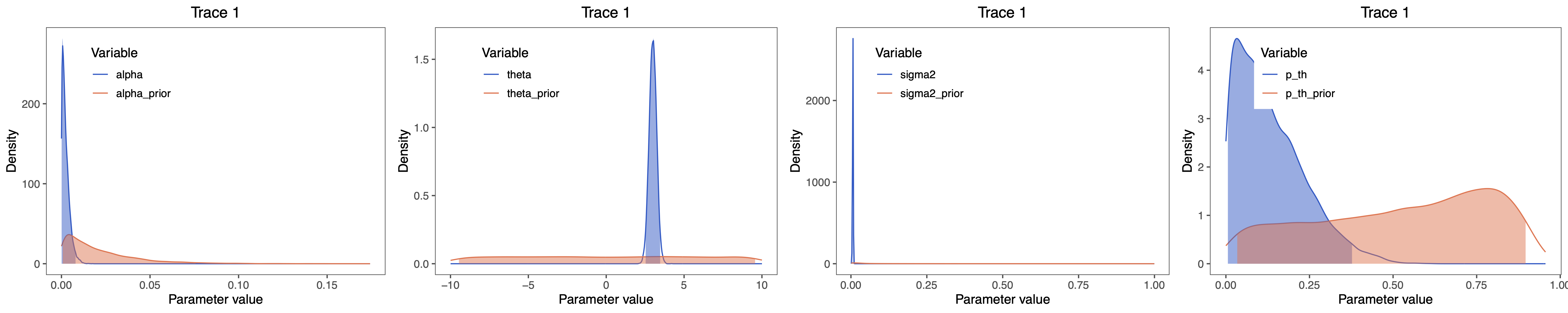
We can plot the posterior estimates of alpha, theta, sigma2, t_half and p_th in RevGadgets. Launch R and use the following code.

First, we need to load the R packages RevGadgets and gridExtra (to arrange the parameters in one plot).

library(RevGadgets)
library(gridExtra)
library(ggplot2)

Next, read the MCMC output:

samples <- readTrace("output/simple_OU.log", burnin = 0.25)[[1]]
samples_OU_prior  <- readTrace("output/simple_OU_prior.log", burnin = 0.25)[[1]]

# combine the samples into one data frame
samples_OU$alpha_prior <- samples_OU_prior$alpha
samples_OU$theta_prior <- samples_OU_prior$theta
samples_OU$sigma2_prior <- samples_OU_prior$sigma2
samples_OU$t_half_prior <- samples_OU_prior$t_half
samples_OU$p_th_prior <- samples_OU_prior$p_th

Next, we create the plot objects:

alpha_plot <- plotTrace(samples, vars="alpha")[[1]] +
              theme(legend.position = c(0.25,0.81))
theta_plot <- plotTrace(samples, vars="theta")[[1]] +
              theme(legend.position = c(0.25,0.81))
sigma_plot <- plotTrace(samples, vars="sigma2")[[1]] +
              theme(legend.position = c(0.25,0.81))
t_half_plot <- plotTrace(samples, vars="t_half")[[1]] + scale_x_log10() +
               theme(legend.position = c(0.25,0.81))
p_th_plot <- plotTrace(samples, vars="p_th")[[1]] +
             theme(legend.position = c(0.25,0.81))

Finally, plot the posterior distribution of the state-dependent rate parameters:

grid.arrange(alpha_plot, theta_plot, sigma_plot, p_th_plot, nrow=1)

⇨ The R file for plotting these posteriors: plot_OU.R

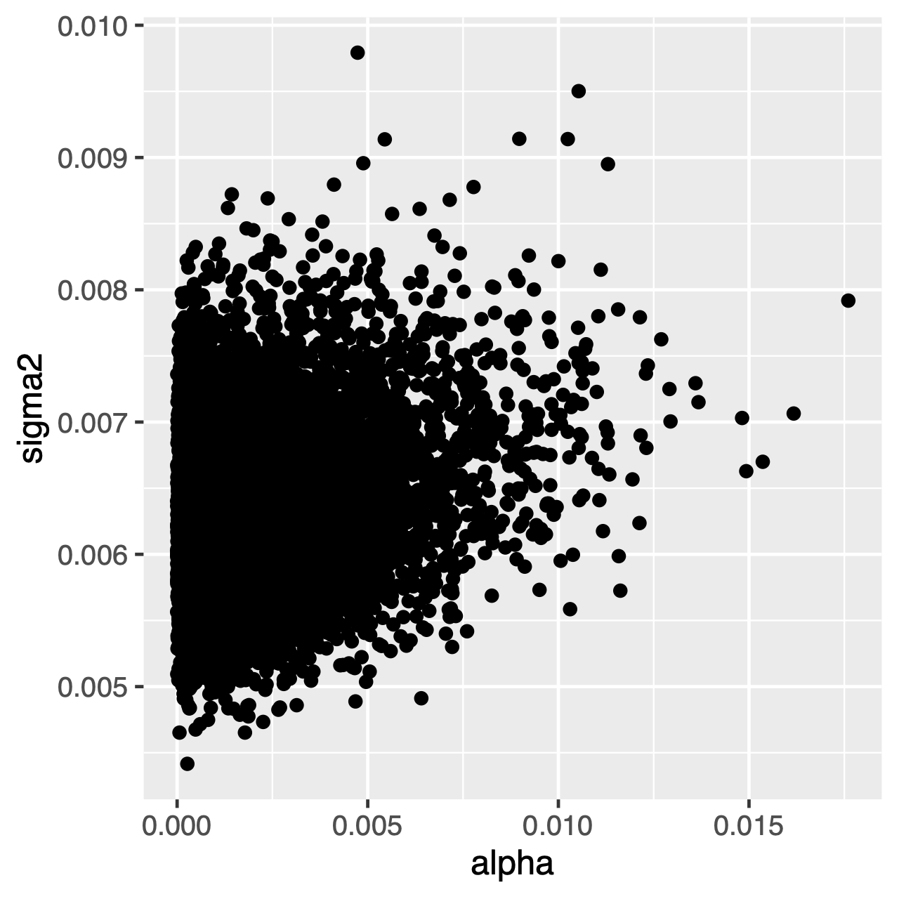
Assessing correlations among parameters

Characters evolving under the OU process will tend toward a stationary distribution, which is a normal distribution with mean $\theta$ and variance $\sigma^2 \div 2\alpha$. Therefore, if rates of evolution are high (or the branches in the tree are relatively long), it can be difficult to estimate $\sigma^2$ and $\alpha$ separately, since they both determine the long-term variance of the process. We can see whether this affects our analysis by examining the joint posterior distribution of the parameters in R, continuing from our previous RevGadgets code. When the parameters are correlated, we should hesitate to interpret their marginal distributions (i.e., don’t make inferences about the rate of adaptation or the variance parameter separately).

library(ggplot2)
ggplot(samples[[1]], aes(x=alpha, y=sigma2)) + geom_point()

⇨ The R file for plotting these posteriors: plot_OU.R

Exercise 1

• Run an MCMC simulation to estimate the posterior distribution of the OU optimum (theta).
• Load the generated output file into RevGadgets: What is the mean posterior estimate of theta and what is the estimated HPD?
• Use R to compare the joint posterior distributions of alpha and sigma2. Are these parameters correlated or uncorrelated?
• Compare the prior mean with the posterior mean. (Hint: Use the optional argument underPrior=TRUE in the function mymcmc.run()) Are they different (e.g., )? Is the posterior mean outside the prior 95% probability interval?

Comparing OU and BM models

Now that we can fit both BM and OU models, we might naturally want to know which model does fits better. In this section, we will learn how to use reversible-jump Markov chain Monte Carlo to compare the fit of OU and BM models.

Model Selection using Reversible-Jump MCMC

To test the hypothesis that a character evolves toward a selective optimum, we imagine two models. The first model, where there is no adaptation towards the optimum, is the case when $\alpha = 0$. The second model corresponds to the OU model with $\alpha > 0$. This works because Brownian motion is a special case of the OU model when the rate of adaptation is 0. Unfortunately, because $\alpha$ is a continuous parameters, a standard Markov chain will never visit states where each value is exactly equal to 0. Fortunately, we can use reversible jump to allow the Markov chain to consider visiting the Brownian-motion model. This involves specifying the prior probability on each of the two models, and providing the prior distribution for $\alpha$ for the OU model.

Using rjMCMC allows the Markov chain to visit the two models in proportion to their posterior probability. The posterior probability of model $i$ is simply the fraction of samples where the chain was visiting that model. Because we also specify a prior on the models, we can compute a Bayes Factor for the OU model as:

where $P( \text{OU model} \mid X)$ and $P( \text{OU model})$ are the posterior probability and prior probability of the OU model, respectively.

Reversible-jump between OU and BM models

To enable rjMCMC, we simply have to place a reversible-jump prior on the relevant parameter, $\alpha$. We can modify the prior on alpha so that it takes either a constant value of 0, or is drawn from a prior distribution. Finally, we specify a prior probability on the OU model of p = 0.5.

alpha ~ dnReversibleJumpMixture(0.0, dnExponential( abs(root_age / 2.0 / ln(2.0)) ), 0.5)

We then provide a reversible-jump proposal on alpha that proposes changes between the two models.

moves.append( mvRJSwitch(alpha, weight=1.0) )

Additionally, we provide the normal mvScale proposal for when the MCMC is visiting the OU model.

moves.append( mvScale(alpha, weight=1.0) )

We include a variable that has a value of 1 when the chain is visiting the OU model, and a corresponding variable that has value 1 when it is visiting the BM model. This will allow us to easily compute the posterior probability of the models because we simply need to compute the posterior mean value of this parameter.

is_OU := ifelse(alpha != 0.0, 1, 0)
is_BM := ifelse(alpha == 0.0, 1, 0)

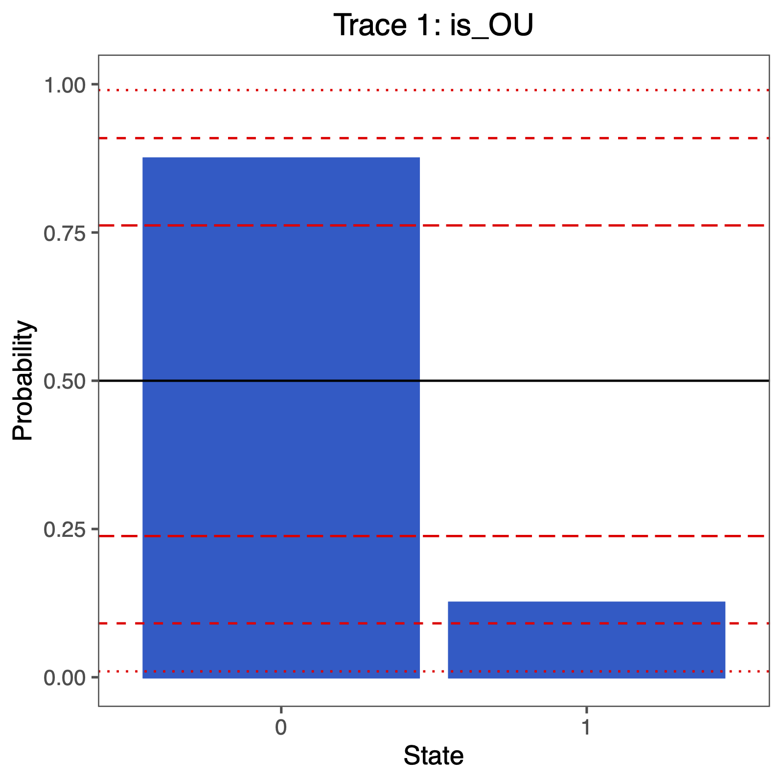
The fraction of samples for which is_OU = 1 is the posterior probability of the OU model. Alternatively, the posterior mean estimate of this indicator variable corresponds to the posterior probability of the OU model. These values can be used in the Bayes Factor equation above to compute the Bayes Factor support for either model.

You can plot the support using the following R code:

library(RevGadgets)
library(ggplot2)

# specify the input file
file <- "output/simple_OU_RJ.log"

# read the trace and discard burnin
trace_qual <- readTrace(path = file, burnin = 0.25)

BF <- c(3.2, 10, 100)
p = BF/(1+BF)
# produce the plot object, showing the posterior distributions of the rates.
p <- plotTrace(trace = trace_qual,
          vars = c("is_OU"))[[1]] +
          ylim(0,1) +
          geom_hline(yintercept=0.5, linetype="solid", color = "black") +
          geom_hline(yintercept=p, linetype=c("longdash","dashed","dotted"), color = "red") +
          geom_hline(yintercept=1-p, linetype=c("longdash","dashed","dotted"), color = "red") +
     # modify legend location using ggplot2
     theme(legend.position = c(0.40,0.825))

ggsave("ou_RJ.pdf", p, width = 5, height = 5)

1. Butler M.A., King A.A. 2004. Phylogenetic comparative analysis: a modeling approach for adaptive evolution. The American Naturalist. 164:683–695.
2. Felsenstein J. 1985. Phylogenies and the comparative method. The American Naturalist.:1–15. 10.1086/284325
3. Hansen T.F. 1997. Stabilizing selection and the comparative analysis of adaptation. Evolution. 51:1341–1351.
4. Höhna S., Heath T.A., Boussau B., Landis M.J., Ronquist F., Huelsenbeck J.P. 2014. Probabilistic Graphical Model Representation in Phylogenetics. Systematic Biology. 63:753–771. 10.1093/sysbio/syu039